Table of contents
Making binary codes from probabilities
Huffman algorithm
Huffman example step by step
 
 

Making binary codes from probabilities

We have a text like "aaabc", with the probabilities you can see below. Because we can output bits, what about if we make a binary decision? the most probable or the rest, 0 or 1. In our example, 0 for 'a', then 1 for the rest, 'b' and 'c', and then we have to choose again: 0 for 'b' and 1 for 'c'. Using that codes we can output "01001110" and the decoder will correctly decode "abacb". That is because the codes have the prefix property and also are instantaneously decodable. Notice too that they are close to the entropy.
 

Symbol	Probability	Code	Entropy (ideal code length)
a	3/5	0 (1 bit)	0.737 bits
b	1/5	10 (2 bits)	2.322 bits
c	1/5	11 (2 bits)	2.322 bits

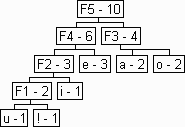
Because we are doing a binary decision, we could represent it with a binary tree. A binary tree is a data structure, whose shape is like a tree (but upside down). It has an starting node called root. The root has two children (pointers to two other nodes), in our case we assign 0 to one child and 1 to the other. If a node has no child it's called a leaf, here it is where there are the symbols. In the example you can see the probability of the node in brackets.

It looks that if we want to assign the right codes, the trick is having similar probabilities at every node. For example if 'a' had a probability of 2, the probabilities at every child of the root wouldl be the same, and the codes would achieve the entropy (a entropy(2/4)=1 bit, b entropy(2/4)=2 bits).

The way to achieve that is making the probability of the current node the sum of the probabilities of its children. That is what the smart David Huffman realized long ago and published in the paper called "A Method for The Construction of Minimum Redundancy Codes" in 1952. In the next section we'll see his method.
 

Huffman algorithm

To achieve optimality Huffman joins the two symbols with lowest probability and replaces them with a new fictive node whose probability is the sum of the other nodes' probabilities (a fictive node is a node that doesn't hold a symbol). The two removed symbols are now two nodes in the binary tree. The fictive node it's their parent and it's not inserted in the binary tree yet. Instead we keep it in the input list. We then repeat the process till the input list is empty. Below you can see a probability distribution and its huffman binary tree.
 

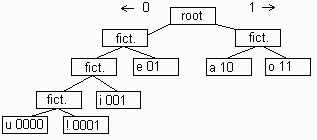
Symbol	Probability	Code	Entropy (ideal code length)
e	3/10	10 (2 bits)	1.737 bits
a	2/10	01 (2 bits)	2.322 bits
o	2/10	11 (2 bits)	2.322 bits
i	1/10	001 (3 bits)	3.322 bits
!	1/10	0001 (4 bits)	3.322 bits
u	1/10	0000 (4 bits)	3.322 bits

Huffman tree with probabilities and Huffman tree showing codes.

In practice we sort the list by the probability (highest probability, first position) instead of searching for the two symbols with lowest probability. That way we can directly get the last two nodes and put them on the output binary tree. When there's only one element left on the input list, the binary tree is done. That node is the root.

Let's see the example shown above step by step.
 

Huffman example step by step

To start with we sort the list. The binary tree is still empty, while the list is full.

LIST:
e 3
a 2
o 2
i 1
u 1
! 1

BT:
...

Now we join the two last symbols into a single one, the fictive node 1 (f1). Then we put those two nodes in the output binary tree. Fictive node 1 points to them (a fictive node is a node that doesn't hold a symbol). Now we sort the list, to be sure that the two last nodes are the ones with lowest probability.

LIST:
e 3
a 2
o 2
f1 2 - u !
i 1

BT:
u 1
! 1

We repeat the same operations. We have now stored the fictive node 1 in the output binary tree. Also have a look at f2: it points to 'i' (a symbol) and to 'f1' (a fictive node).

LIST:
e 3
f2 3 - f1 i
a 2
o 2

BT:
f1 2 - u !
i 1
u 1
! 1

The pointers in a fictive node point to the binary tree.

LIST:
f3 4 - a o
e 3
f2 3 - f1 i

BT:
a 2
o 2
f1 2 - u !
i 1
u 1
! 1

Fortunately we have algorithms and loops which do such repetitive task for us.

LIST:
f4 6 - f2 e
f3 4 - a o

BT:
e 3
f2 3 - f1 i
a 2
o 2
f1 2 - u !
i 1
u 1
! 1

And the last step. There's only one node left in the input list. This is the root, the start of the binary tree.

LIST:
f5 10 - f4 f3

BT:
f4 6 - f2 e
f3 4 - a o
e 3
f2 3 - f1 i
a 2
o 2
f1 2 - u !
i 1
u 1
! 1

Now let's see what our binary tree looks like.